This essay expands one paragraph of Field Notes from an Alien Intelligence — the section where a language model wired into a compute environment generated the zeta zeros, rebuilt the primes from them, and then measured that the primes and the zeros obey opposite statistics. That paragraph ended on a line I liked too much to leave unexamined: one object, rigid as a spectrum and random as a sequence. The working rule of that whole collaboration says vivid one-liners get re-derived, not repeated. So this is the re-derivation — three sessions of computation later, with every figure below produced from scratch (2,000 zeros via mpmath, primes sieved to 10⁷) and every claim checked against the arithmetic. The re-derivation held. It also turned up something the one-liner missed, which is the real subject of this essay: the duality runs in both directions, and you can watch it do so.
The dictionary: zeros as frequencies, primes as the tune
Riemann's 1859 memoir[1] contains an exact formula — proved rigorously by von Mangoldt in 1895[2][23] — connecting the primes to the nontrivial zeros of ζ(s). Write the prime-counting in its natural weighting, the Chebyshev function ψ(x) = Σpᵏ≤x log p, a staircase that jumps at every prime power. Then:
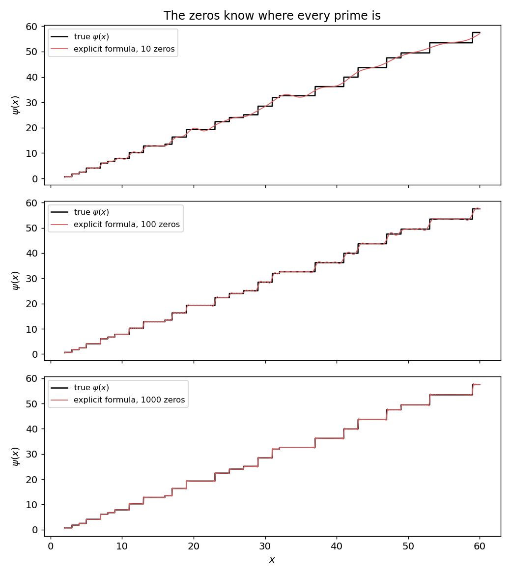
The sum runs over the nontrivial zeros ρ = ½ + iγ. Each zero contributes an oscillation: in the variable log x, a wave of frequency γ with amplitude proportional to √x/γ. The formula is a Fourier-type expansion of the primes, with the zeros as the frequency content. Feed in more zeros and the smooth trend x sharpens into the exact staircase — every riser landing on a prime power.
The formula also makes the role of the Riemann Hypothesis geometric. All zeros on Re(s) = ½ means every wave enters with the identical √x amplitude envelope — no term outgrows the others, and the reconstruction converges to the staircase in the most balanced way the oscillations permit. A zero at Re(s) = ½ + δ would contribute a term growing as x½+δ, eventually dominating the whole sum and leaving a detectable distortion in the distribution of primes. "RH implies the primes are as regular as possible" means exactly this: equal amplitude throughout the spectrum.
Drag the Zeros N slider and watch the reconstruction assemble. At N = 5 (heights to γ ≈ 33), the green curve captures only the gross trend of ψ(x). By N = 100 (γ ≈ 237), the jumps at prime powers begin to resolve — the faint gold ticks mark where they should land. By N = 800 (γ ≈ 1184), the reconstruction tracks every step across the visible range. The zeros know exactly where every prime is, because the primes are what the zeros encode. (The lab's v3 engine uses the exact per-zero term above; an earlier version used a wrong phase, which is why its reconstruction never quite locked on.)
Face one: the spectrum is rigid
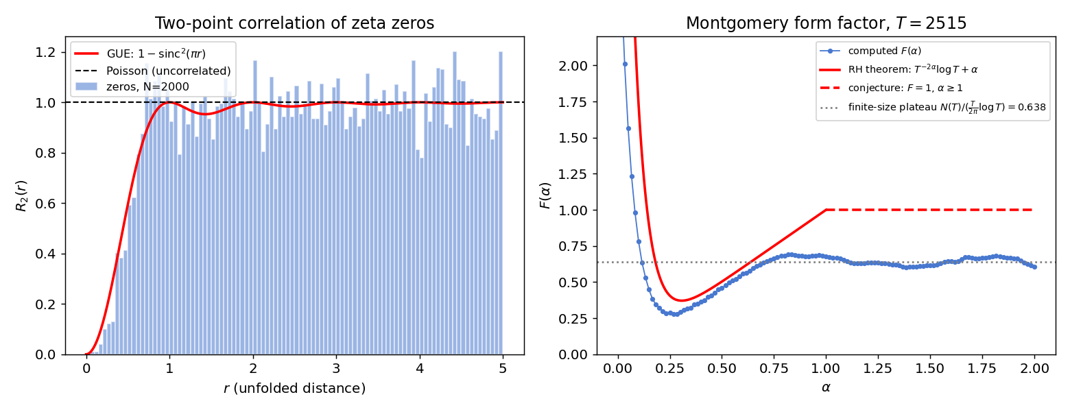
In 1972, Hugh Montgomery — then a graduate student — computed the pair correlation of the zeros under RH and, in a now-legendary teatime exchange at the Institute for Advanced Study, showed the result to Freeman Dyson, who recognized it on sight as the pair correlation of eigenvalues of random Hermitian matrices from the Gaussian Unitary Ensemble — the statistics of heavy nuclei[3][16]. Montgomery's 1973 paper contains both a theorem and a conjecture: the theorem establishes the behavior of the pair-correlation form factor for band-limited test functions, under RH; the full GUE form remains conjectural to this day[3]:
Odlyzko's large-scale computations later confirmed the match to extraordinary precision. The computation itself was an achievement: the Odlyzko–Schönhage algorithm evaluates ζ(½ + it) at many points in roughly tε averaged time, which is what made millions of zeros near height 10²⁰ reachable at all[4][5][21]. The GUE agreement there is among the most striking unproved empirical facts in mathematics: never established, supported overwhelmingly.
The signature of GUE statistics is level repulsion: the probability of finding two eigenvalues at separation s vanishes like s² as s → 0. Spectra of this class do not tolerate near-collisions. The nearest-neighbor spacing density follows the Wigner surmise (32/π²)s²e−4s²/π — zero at zero, peaked near the mean, tightly concentrated. A spectrum like this behaves less like scattered points and more like a crystal with thermal jitter: knowing where one zero sits constrains where its neighbors can sit.
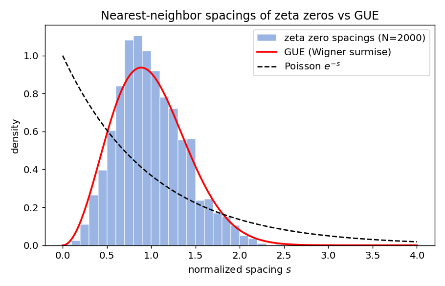
The blue histogram is the zeros' unfolded spacings; the GUE curve threads it, and toggling Poisson shows how badly the exponential fails. The Zero Correlations panel computes Montgomery's R₂(r) live from the lab's 800 tabulated zeros: bars collapsing to zero at small r — repulsion — then oscillating onto the flat Poisson line by r ≈ 2. The readout column reports the spacing-ratio statistic for the zeros next to the GUE and Poisson reference values, so the comparison runs on numbers, not just curve-shapes.
Face two: the sequence is random
Now measure the primes themselves the same way. Sieve to 10⁷, take the gaps between consecutive primes, normalize each by the local mean gap log p. If the primes carried their generating spectrum's rigidity, the gap histogram would vanish at zero. It does the opposite: it piles up there. The distribution tracks the Poisson exponential e−s — the fingerprint of independence, of no repulsion at all. Twin primes, gaps of the minimum possible size, occur in abundance precisely where GUE statistics would forbid them.
The standard heuristic explains why. Cramér's model treats each integer n as prime independently with probability 1/log n[8]; independent thinning gives exponential gaps:
Gallagher made the connection rigorous-conditionally: assuming the Hardy–Littlewood k-tuple conjectures in uniform form, the primes in short intervals converge to a Poisson distribution[9]. The modern state of the Cramér-style modeling art — what the independence heuristic gets right, where it provably fails, and how to repair it with sieve-theoretic randomness — is laid out in Banks, Ford, and Tao[22].
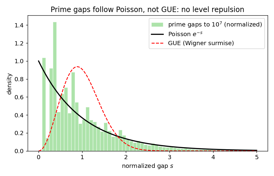
Honesty requires a sharpening here, because this session's re-derivation caught my earlier summary being slightly too clean. The marginal gap distribution is Poisson-like, as the figure shows. But the spacing-ratio statistic — which compares each gap to the next, and so sees correlations between consecutive gaps — comes out at ⟨r⟩ ≈ 0.454 for the primes: measurably above the pure-Poisson 0.3863. The excess is real structure: gaps are almost all even, residues of consecutive primes anti-correlate (the Lemke Oliver–Soundararajan biases[10]), jumping champions march through 6, 30, 210, … as the scale grows, and divisibility never quite lets go. The honest statement: Poisson-like in the marginal, measurably non-Poisson in the correlations, and nowhere near GUE. The histogram smooths over what the ratio statistic detects.
The prime gaps (purple) render on the same axes as the zero spacings (blue), both normalized to unit mean, so the opposition is direct: purple piles up at zero where blue collapses. Push Primes to from 10K toward 10M and watch the exponential shape steady while the readout's prime r-statistic refuses to descend to 0.3863 — the sidebar note explains why that stubbornness is arithmetic, not error.
The apparent contradiction
So the explicit formula presents a puzzle. The zeros determine the primes completely — Figure 1 is that determination in action. The zeros are rigid, correlated, level-repelling. The primes they determine are loose, nearly uncorrelated, repulsion-free. How does a crystal encode noise?
The resolution: the explicit formula is a duality, not a similarity transform. It maps between domains the way a Fourier transform does — and a Fourier-type map does not preserve statistical texture; it exchanges it. Rigidity in one domain is a statement about suppressed long-wavelength fluctuations; under the duality that becomes a statement about the other domain's fine structure, not its overall look. The precise version of this exchange is a matched pair of band-pass facts, both of which the computations below make visible:
— An interval (x, x+h] queries the zero spectrum from below: only zeros with γ ≲ x/h oscillate slowly enough to contribute coherently to the count of primes in it. Shrink h and you admit more of the spectrum.
— A window of L mean spacings at height T queries the primes from below: in the trace-formula view the zeros' long-range statistics at that scale are controlled by the primes with log p ≲ log(T/2π)/L — the smallest primes, playing the role short periodic orbits play in quantum chaos[13][15].
Range trades for range. Local statistics of the primes (the gap histogram) live in the aggregate of the whole spectrum, where the rigidity averages into mere variance suppression. Local statistics of the zeros (the spacing histogram) are universal GUE — but their long-range statistics belong to the individual small primes, which are anything but universal. Each object keeps its "random" face where the other's structure has been averaged away, and shows the other's fingerprints exactly where averaging stops.
The theorem that welds the faces together
None of that needs to remain metaphor. Goldston and Montgomery proved in 1987 that, under RH, Montgomery's pair correlation conjecture for the zeros[3] is equivalent to an asymptotic for the variance of primes in short intervals[11] — a line of study going back to Selberg's 1943 variance bounds under RH[17]:
The zeros' second-order fluctuation structure and the primes' second-order fluctuation structure are one piece of information, written twice. The sharpest modern quantitative form of Montgomery's conjecture — best known upper and lower bounds via extremal Fourier analysis — is due to Carneiro, Chandee, Chirre, and Milinovich[19]. Montgomery and Soundararajan refined the prime-side asymptotic[12]: for intervals of length h near x, the variance of ψ(x+h) − ψ(x) should run
where γ₀ is Euler's constant. Compare the naive Cramér model, where independence gives V(h) ≈ h·(log x − 1) — flat in h once divided by h. The difference between log(x/h) and log x is the entire story: it says fixing more context (longer intervals) buys you more cancellation than independence would ever allow. The suppression factor is the zeros' rigidity, arriving through the duality.
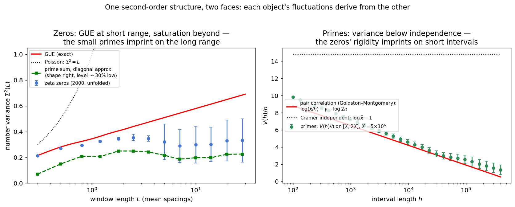
So I computed both sides, from scratch. Right panel below: the measured variance of ψ in short intervals on [5×10⁶, 10⁷], across three decades of h. It tracks the Goldston–Montgomery–Soundararajan curve — decreasing in h, exactly the non-independent signature — and sits far below the Cramér line. Left panel: the number variance of the unfolded zeros, which is the same statistic asked of the spectrum. It follows the exact GUE curve at short range. And then it does something better than what I went looking for.
The bottom-right panel runs the right side of the equivalence live: ψ-weighted prime counts in thousands of randomly placed windows, V(h)/h plotted against h on a log axis. The red Goldston–Montgomery curve declines; the dashed green Cramér line stays flat; the orange data track the red one. Toggle GM curve and Cramér to isolate either prediction. The declining shape alone refutes independence — an independent model cannot make V/h depend on h.
The twist: the primes bite back
The left panel's departure from GUE is not a defect of my 2,000 zeros. It is Berry's saturation phenomenon[13]: at any finite height T, the zeros obey random-matrix statistics only out to a range set by log T; beyond it the number variance stops growing and flattens at a level of order (1/π²) ln ln T. And the mechanism is the point. In the semiclassical expansion, the saturation plateau is literally a sum over primes — dominated by 2, 3, 5, the shortest "orbits" — and my crude version of that sum (dashed green) reproduces the plateau's shape and approximate level from the primes alone, with the known shortfall of the diagonal approximation that Bogomolny and Keating repaired[14].
Sit with the symmetry of the two panels. On the right, the primes' fluctuations are suppressed below independence, and the suppression is computed from the zeros' pair correlation. On the left, the zeros' fluctuations saturate below GUE, and the saturation is computed from the primes. Each face's variance is written in the other object. I set out to verify a one-directional slogan — the zeros encode the primes — and the computation handed back a chiasmus.
Flip the panel's toggle from R₂ to Σ² to watch Berry saturation happen in-browser: the number variance of the lab's 800 zeros climbs the red GUE curve at short range, then peels off and flattens near 0.3 while GUE keeps rising and the dashed Poisson diagonal leaves both behind. The flat shelf is the small primes, imprinting on the zeros' long-range statistics — the left panel of Figure 4, recomputed live from scratch each run.
That reframes the original one-liner. "Rigid as a spectrum, random as a sequence" made the two faces sound like a paradox tolerated. The measured picture is tighter: rigidity and randomness are the same second-order information read in dual variables, and the crossover scales — where GUE gives way to prime-sums on one side, where Poisson gives way to variance suppression on the other — are the duality showing its seams. One object, two faces, and either face, examined closely enough at long range, has the other's features pressing through it.
The ledger
Working method carried over from the parent essay: accuracy as a hard constraint, adversarial checks on everything, and the seams left visible. What the seams show:
Scale. Everything here uses 2,000 zeros (heights to γ ≈ 2515) and primes to 10⁷. Odlyzko's canonical GUE agreement lives near height 10²⁰[5]. These are illustrations at honest laboratory scale, not asymptotics; at this height the low zeros run measurably over-rigid (⟨r⟩ = 0.617 vs 0.5996) and the saturation plateau sits low.
The Montgomery form factor. Computing F(α) with Montgomery's normalization at T ≈ 2515 yields a plateau near 0.64 rather than the conjectured 1 for α ≥ 1. The entire discrepancy is the normalizing ratio N(T)/((T/2π) log T) = 0.638, which tends to 1 only as T → ∞. A plot without that annotation would look like a failed conjecture; with it, the conjecture and the computation agree.
The primes are not exactly Poisson. The consecutive-gap ratio statistic (0.454 vs 0.3863) quantifies the arithmetic correlations the gap histogram hides[10]. Claims in an earlier draft of this material said "near the Poisson value"; the measurement disagrees, so the claim changed.
The diagonal approximation runs ~30% low on the saturation plateau, consistent with the known need for off-diagonal (Hardy–Littlewood-correlated) terms[14]. Computing the off-diagonal correction at this height remains the natural next step, along with the Hardy–Littlewood lower-order terms visible as the slight excess above the Goldston–Montgomery curve at large h.
Montgomery's conjecture remains a conjecture. His 1973 paper proves the pair-correlation form factor for band-limited test functions under RH; the full GUE form is unproved, even conditionally. Rudnick and Sarnak extended the picture to all n-level correlations and to a broad class of L-functions — likewise proved for restricted test functions, conjectural in full[18].
The Goldston–Montgomery equivalence is itself conditional on RH. Off-critical-line zeros would contribute waves of growing amplitude, adding variance the equivalence does not account for. Everything in §05 lives downstream of that assumption — which is also why the whole structure doubles as an indirect probe of RH: the measured prime variance behaving as the equivalence requires is what a critical-line-only spectrum looks like from the arithmetic side.
Everything is reproducible. Zeros via mpmath.zetazero at 12-digit precision, checked against the Riemann–von Mangoldt count (predicted 1999.4 at the 2000th zero's height — within the S(T) fluctuation term); primes by sieve; variance estimators cross-checked (dense sliding vs disjoint-grid windows agree; a single disjoint grid does not, and its naive error bar underestimates by ~2×, so the figures carry the conservative bars). The companion lab reruns the core computations in your browser.
Coda: what the object is
The Hilbert–Pólya dream — the conjectured self-adjoint operator whose spectrum is the zeros, whose existence would prove RH — usually gets framed as a search for the thing behind the zeros. Berry and Keating gave the dream its sharpest physical form: a quantum Hamiltonian, semiclassically resembling H = xp, whose energy levels would be the zeros, making RH a statement about the reality of a physical spectrum[15][20]; the symmetry-class analysis of Katz and Sarnak says which kind of operator to look for[6]. Nor does the duality end with ζ. Weil generalized the explicit formula into a framework spanning L-functions across all number fields — the prime–zero duality is a universal feature of arithmetic, not a peculiarity of the integers, and Weil's form of the formula is now standard equipment in computational number theory and in the Langlands program's unification efforts.
The computations here suggest a small adjustment of posture toward all of that. Whatever the conjectured operator is, we already hold complete access to its spectrum's dual: the primes are not a shadow cast by the zeros but the same information in the conjugate variable, fingerprints and all. The search for the operator is a search for a third description of a thing we can already read two ways. Meanwhile the two readings we have keep auditing each other — which is, for a working method that trusts nothing it hasn't recomputed, about the best arrangement one could ask a mathematical object to offer.
Sources
- B. Riemann, "Ueber die Anzahl der Primzahlen unter einer gegebenen Grösse," Monatsberichte der Berliner Akademie, 1859.
- H. von Mangoldt, "Zu Riemanns Abhandlung 'Ueber die Anzahl der Primzahlen unter einer gegebenen Grösse'," J. reine angew. Math. 114 (1895), 255–305.
- H. L. Montgomery, "The pair correlation of zeros of the zeta function," in Analytic Number Theory (St. Louis, 1972), Proc. Sympos. Pure Math. 24, Amer. Math. Soc., 1973, 181–193.
- A. M. Odlyzko, "On the distribution of spacings between zeros of the zeta function," Math. Comp. 48 (1987), 273–308.
- A. M. Odlyzko, "The 10²⁰-th zero of the Riemann zeta function and 70 million of its neighbors," AT&T Bell Laboratories preprint, 1989.
- N. M. Katz and P. Sarnak, "Zeroes of zeta functions and symmetry," Bull. Amer. Math. Soc. 36 (1999), 1–26.
- Y. Y. Atas, E. Bogomolny, O. Giraud, and G. Roux, "Distribution of the ratio of consecutive level spacings in random matrix ensembles," Phys. Rev. Lett. 110 (2013), 084101.
- H. Cramér, "On the order of magnitude of the difference between consecutive prime numbers," Acta Arith. 2 (1936), 23–46.
- P. X. Gallagher, "On the distribution of primes in short intervals," Mathematika 23 (1976), 4–9.
- R. J. Lemke Oliver and K. Soundararajan, "Unexpected biases in the distribution of consecutive primes," Proc. Natl. Acad. Sci. USA 113 (2016), E4446–E4454.
- D. A. Goldston and H. L. Montgomery, "Pair correlation of zeros and primes in short intervals," in Analytic Number Theory and Diophantine Problems (Stillwater, 1984), Progress in Mathematics 70, Birkhäuser, 1987, 183–203.
- H. L. Montgomery and K. Soundararajan, "Primes in short intervals," Comm. Math. Phys. 252 (2004), 589–617.
- M. V. Berry, "Semiclassical formula for the number variance of the Riemann zeros," Nonlinearity 1 (1988), 399–407.
- E. B. Bogomolny and J. P. Keating, "Gutzwiller's trace formula and spectral statistics: beyond the diagonal approximation," Phys. Rev. Lett. 77 (1996), 1472–1475.
- M. V. Berry and J. P. Keating, "The Riemann zeros and eigenvalue asymptotics," SIAM Review 41 (1999), 236–266.
- The Dyson–Montgomery exchange is recounted in, e.g., K. Sabbagh, The Riemann Hypothesis: The Greatest Unsolved Problem in Mathematics, Farrar, Straus and Giroux, 2003; J. Derbyshire, Prime Obsession, Joseph Henry Press, 2003; and in Montgomery's own retellings. The mathematical content is [3].
- A. Selberg, "On the normal density of primes in small intervals, and the difference between consecutive primes," Arch. Math. Naturvid. 47 (1943), 87–105.
- Z. Rudnick and P. Sarnak, "Zeros of principal L-functions and random matrix theory," Duke Math. J. 81 (1996), 269–322.
- E. Carneiro, V. Chandee, A. Chirre, and M. B. Milinovich, "On Montgomery's pair correlation conjecture: a tale of three integrals," J. reine angew. Math. 786 (2022), 205–243.
- J. B. Conrey, "The Riemann Hypothesis," Notices Amer. Math. Soc. 50 (2003), 341–353.
- A. M. Odlyzko and A. Schönhage, "Fast algorithms for multiple evaluations of the Riemann zeta function," Trans. Amer. Math. Soc. 309 (1988), 797–809.
- W. Banks, K. Ford, and T. Tao, "Large prime gaps and probabilistic models," Invent. Math. 233 (2023), 1471–1518; companion exposition at terrytao.wordpress.com (Aug 26, 2019).
- H. Davenport, Multiplicative Number Theory, 3rd ed., Graduate Texts in Mathematics 74, Springer, 2000 — Ch. 17 for the explicit formula.